PLASIMO uses structured meshes for discretizing the equations. The mesh can be equidistant or stretched. The supported coordinate systems in PLASIMO are:

Cylindrical coordinates

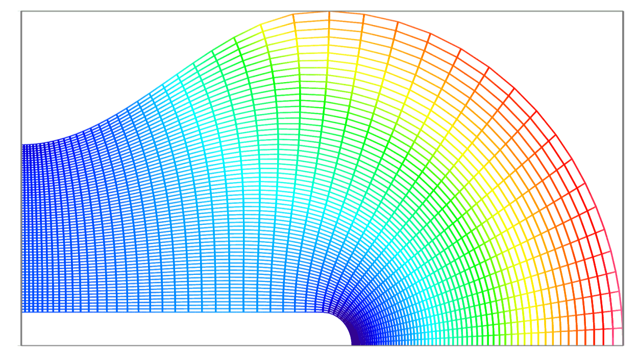
Apart from the usual \((r,z)\) cylindrical grid with azimuthal symmetry, PLASIMO provides \((r,\phi)\) cylindrical grid with symmetry coordinate \(z\).

Cylindrical coordinates \((r,z)\) with azimuthal symmetry.

Cylindrical coordinates \((r,\phi)\) with axial symmetry.

Spherical coordinates

3D spherical coordinates. The figure shows the simulations planes in the three directions.

Prolate spheroidal coordinates

The prolate spheroidal coordinates are useful for modeling of pin-to-plate electrode configuration or tip-to-tip configuration. More information about the definition can be found in Wikipedia: Prolate-spheroidal-coordinates.

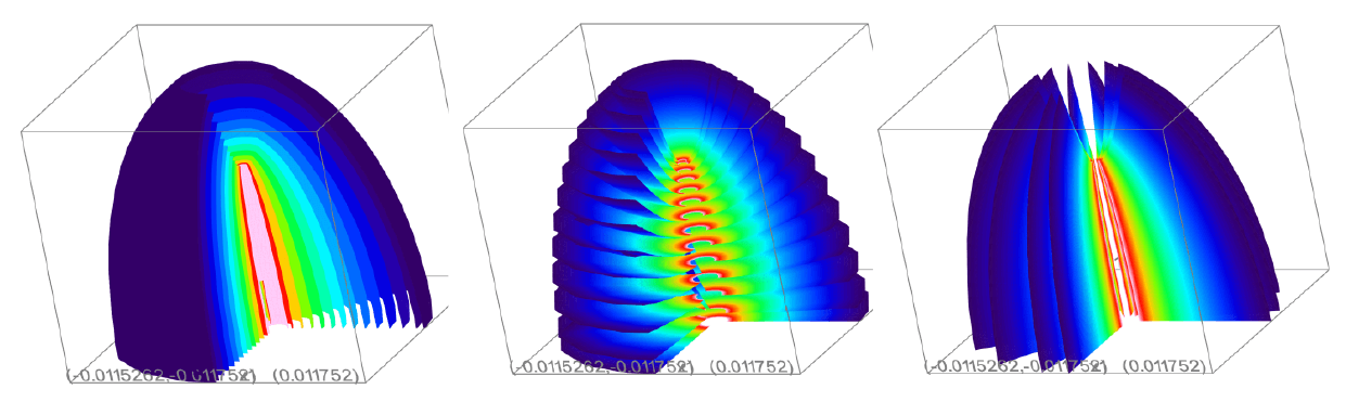
Temperature field calculation on prolate spheroidal coordinates. The figures show the simulation planes in the three directions.

User-defined coordinates

In case the appropriate coordinate system is not predefined in PLASIMO, PLASIMO gives the option any coordinate system to be defined by specifying the parametric functions \(x, y\) and \(z\) for the coordinates and \(L_1, L_2\) and \(L_3\) for the scale factors. The screenshot below shows a specification of user-defined bipolar coordinates (Bipolar).

Examples of user-defined coordinate systems:

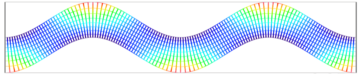
Bipolar coordinates

2D elliptic coordinates

Ortho-curvilinear coordinate systems

PLASIMO uses ortho-curvilinear (OCL) coordinate systems. OCL are characterized by curved coordinate lines with the property that at locally the two coordinate lines intersect perpendicularly. The location of the grid points of an OCL grid are determined by the boundary prescription. The boundary curves are specified by their parametric functions.